Architectural Colour Schedule in Excel

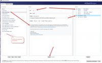
The last post I tried to use AirTable to create a Colour Schedule from a Revit export. Thinking I could use the Database to cross reference items in the room such as doors/windows etc to be able to pull those in to make the colour scheme planning more comprehensive. It didn’t work.

Along the way from transferring data from Revit to AirTable it had to be passed through a CSV/XLX file format to get from one to the other and back again. So I thought, do the colour scheme in the spreadsheet instead.

I had previously used Conditional formatting in Excel for condition over time so that you could filter building components by year based on their condition, this would allow you to forecast what work was coming up in the following years. See this example and this article.

What I was looking for was a way to reference selected materials and describe them adequately for a schedule and be able to do a simple colour comparison to see that all the elements were in the correct colour range I’d selected.

Process

For copy of Excel Workbook click on LINK

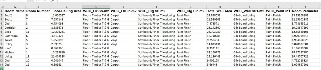
I initially just did an extract from a 3D PDF of my house and dropped the data into my excel sheet to get data on room finishes. Its pretty simple, it just has rooms, areas, base material and finish.

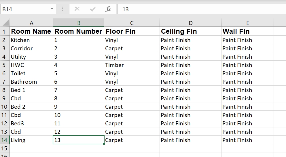
I then cleaned this up, because I only really wanted finishes, so the table was reduced to:

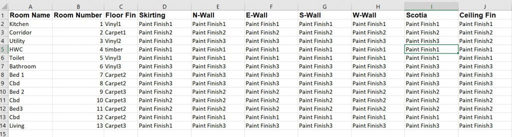
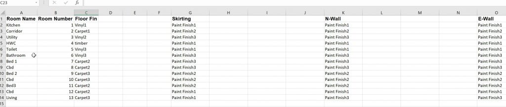
I also wanted 4 faces of walls for rooms, as well as skirting & scotias, so I added these columns in. I also changed some of the references, so instead of Vinyl, there would be different types, as well as paint finishes, carpets etc

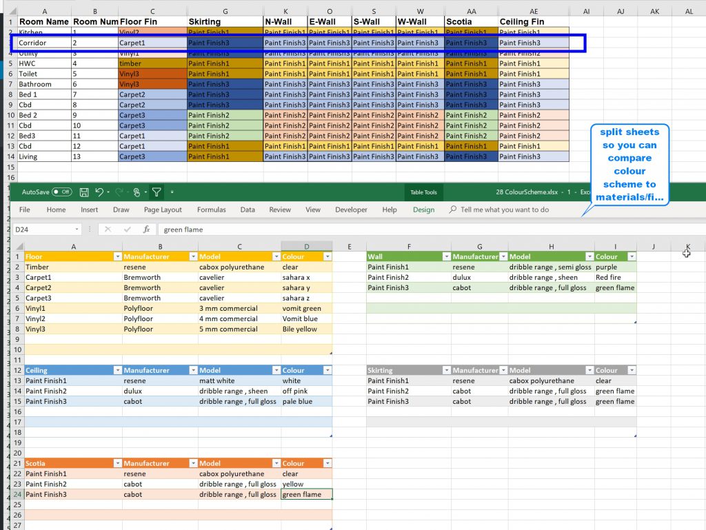
So, now I want a list of finishes for these elements, so I make another sheet as follows:

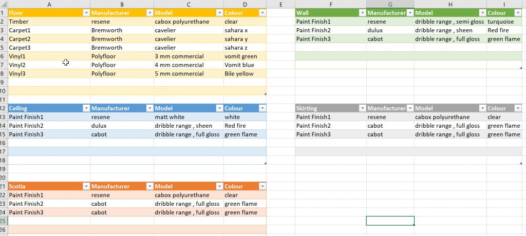
So there is a separate Sheet with tables for each Element, with possible materials/models/colours relating to that element. You could put this at the bottom of your initial worksheet, but I’ve just put it on another sheet to keep it tidy. If you need to compare later, you can always split the screen and show both sheets.

In the first sheet we will add 3 blank columns (for manufacturer/model/Colour) between each of the current finishes columns

Using Vlookup() in Excel

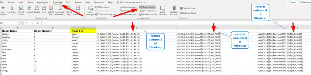
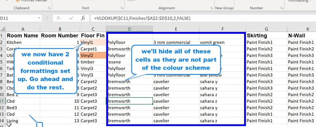
So, in floors , the first active room cell is C2, this holds the material for floor finish. So in Cell D2 we want to be able to lookup the manufacturer for this type of vinyl. We will use the Vlookup() excel function to look to cell C2 on this sheet, compare it to the Floor Finishes table on the next sheet over, when it gets a correct comparison on that table, it will fill in the result of the next column along, which is the manufacturers column.

The video below demonstrates how you use Vlookup:

so the function in cell D2 looks like this:

=VLOOKUP($C2,Finishes!$A$2:$D$10,2,FALSE)

The $ sign in front of each cell code, of say cell =C2, means that if you have =$C$2 this means this is an a ABSOLUTE CELL REFERENCE , so if you copy that formula by dragging the formula down or across the spreadsheet, that part of the formula will always reference only that cell =$C$2.

If you just had just =C2 and you dragged that down to the next row (or copied/pasted) then it would read =C3 instead, so it would be a RELATIVE CELL REFERENCE, not an ABSOLUTE CELL REFERENCE.

So, now we can use the formula above that says:

=VLOOKUP($C2,Finishes!$A$2:$D$10,2,FALSE)

Look in Cell C2 and then look up that reference in the table on the finishes sheet and find the corresponding match. When you find it, in column 1 of that table, return to me the value in the 2nd column over on that row (this is Manufacturer). The last FALSE means it must be an absolute match, or don’t return anything (#N/A).

The #N/A would occur if you created in the finishes schedule a type Vinylx (you miss-typed it), there would not be an equivalent in the floor table so you get a Not applicable N/A. So go check your spelling.

For the next column along, to get make, all we have to do is change the 2 for a 3, as below

=VLOOKUP($C2,Finishes!$A$2:$D$10,3,FALSE)

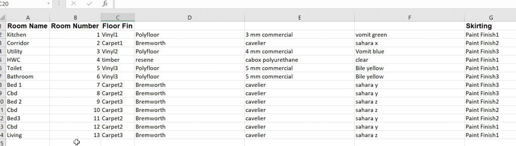
So this has now populated our floor finishes room list with specific materials and finishes. If we change the name of the column from Vinyl1 to Vinyl2 then all the data will change in the next 3 columns, so we are specifying the correct product/material/finish

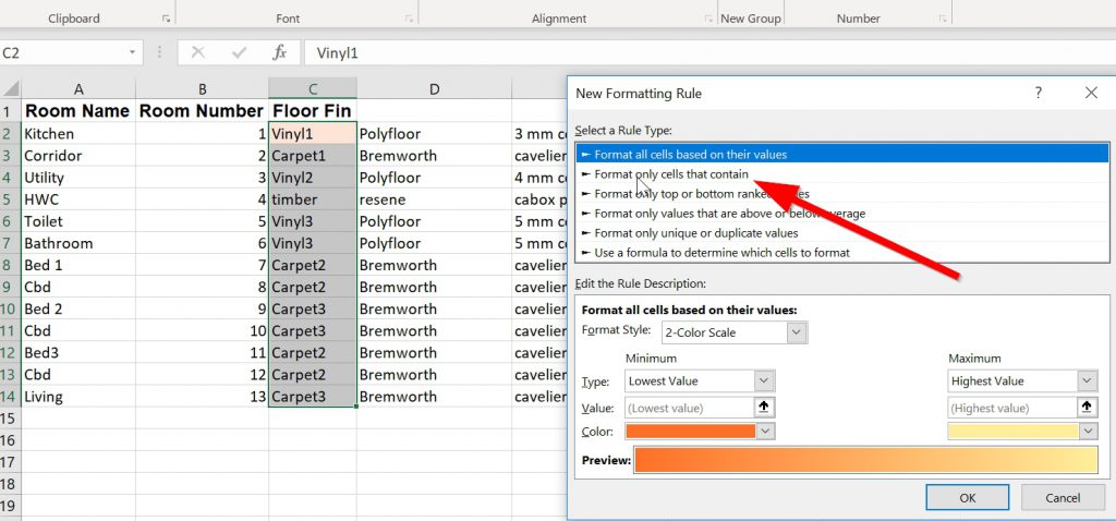
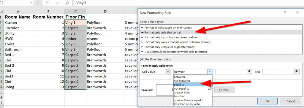
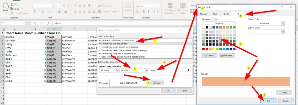
Show it in colour- Conditional formatting

So we can copy the formula across and populate all the other columns, then we can hide the manufacturer/model/colour columns as we know they are populating correctly.

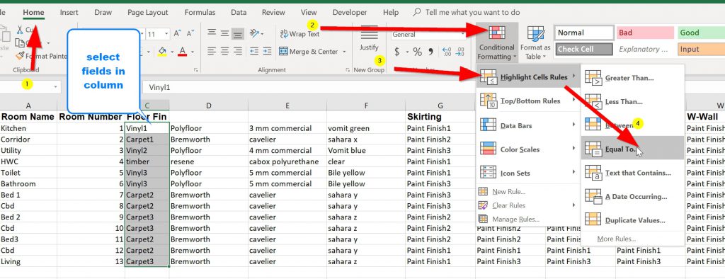
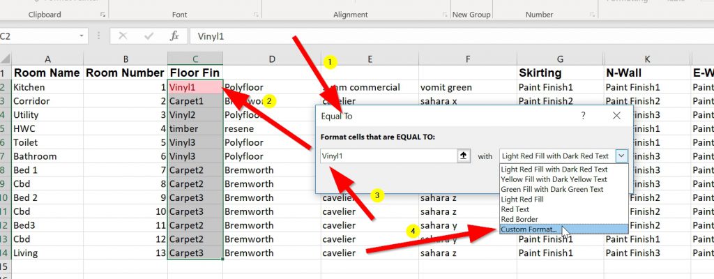
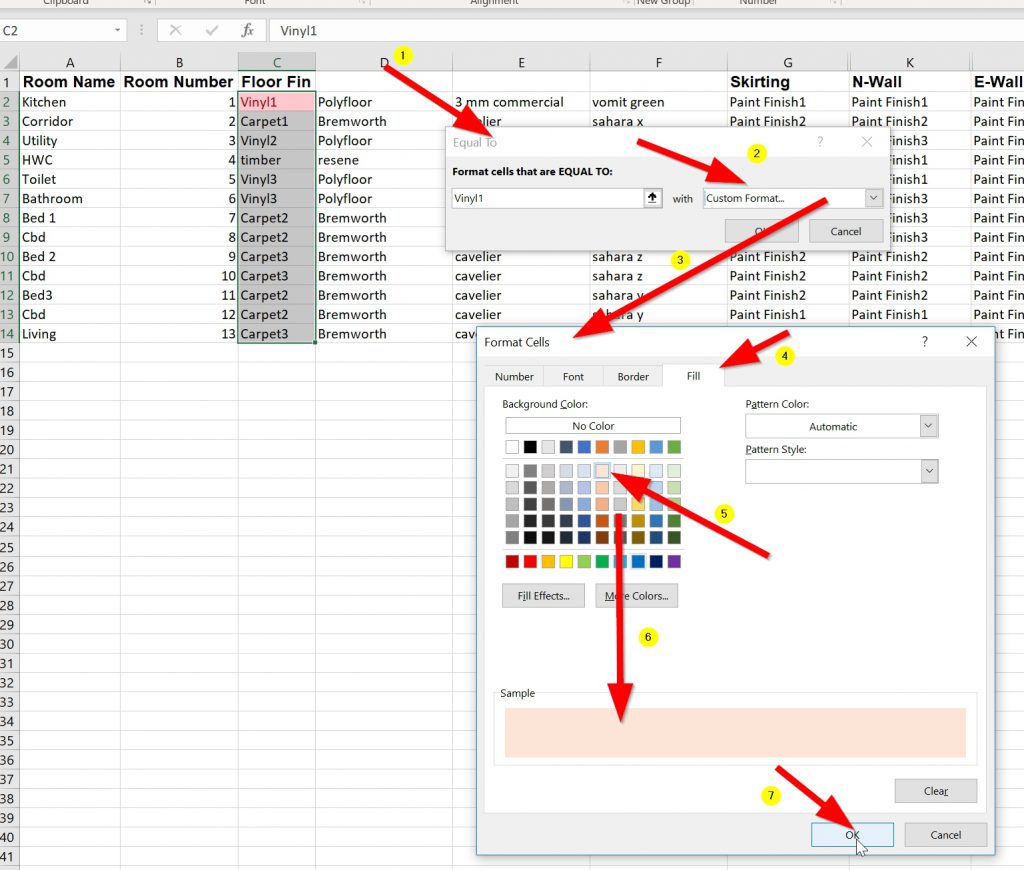
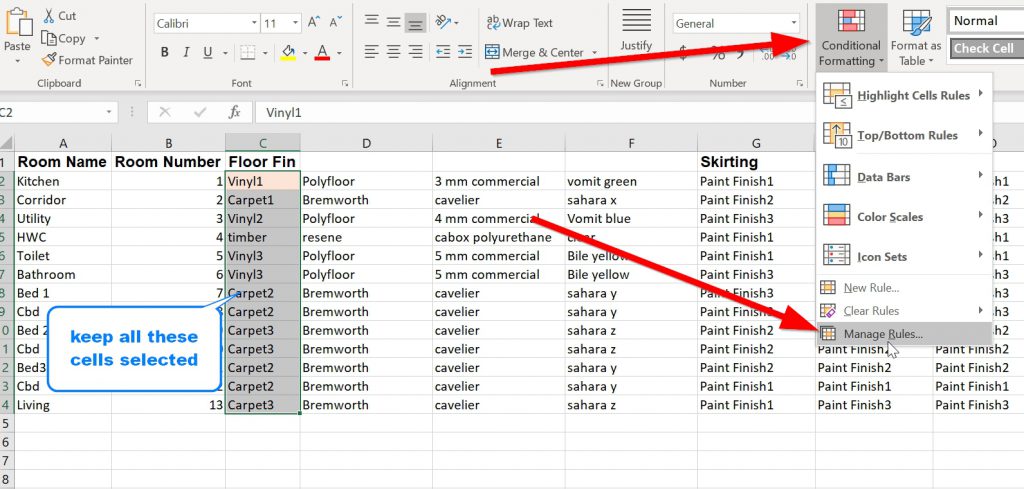
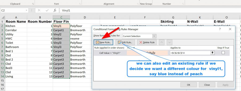
The process above can be repeated, or else, as we have one setup now, we can go int the MANAGE RULES of the Conditional Formatting tab

The result

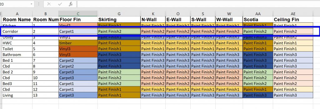
Using the setup above, I have highlighted the Corridor. The colours do not seem to be too good with blues, greens and peach colours.

So we can start to adjust them by selecting other finishes from the list so that they look more harmonious.

To help with the referencing we can have the sheet with the tables to show what we are using. We can always adjust the Manufacturer/Model/Colour to suit our needs.

A further thing I’d add to all the finishes is a comments column, so if you wanted something special, like a feature pattern or something that was specific to that item, then you could reference it in the “Comments” field.

This is only a method of getting data into Excel to manipulate the colour scheme, or test a number of Schemes. You could create 2 more sheets, your colour scheme sheet and your tables sheet and then create a 2nd colour scheme. You could use FIND/REPLACE to change the vlookup reference sheet from Finishes to say Finishes2. This keeps all your original setup, you just need to change the colours in your conditional formatting.

=VLOOKUP($C2,Finishes!$A$2:$D$10,2,FALSE) to
=VLOOKUP($C2,Finishes2!$A$2:$D$10,2,FALSE)

Getting data back into Revit

Several ways to transfer data to/from Revit. You would need to have a Revit Schedule for say floor, walls, etc , they could be separate category schedules, then you need to map the Excel finishes floor to a separate sheet that has the same column headers as the revit schedule, then Export the Revit schedule using BIMOne Export/Import Excel and copy Values from linked sheet.

End thoughts

I am pleased with the result. After trying it in AirTable , then in LibreOffice, in which I had problems with their styles, not as intuitive as I’d thought, just switching from Excel, which I’m used to.

Once I’d got the principles of what I was trying to do the process was pretty straight forward. It took a little while to setup, specifically the colour filters but once they were up and running it was easy to adjust.

It would have been nice to colour all the fields (inc Manufacturer/Model/Colour) but in some ways compressing it makes it easier to view.

I will think about the process as I think you could use macros to speed up some of the steps, maybe even templating part of the process would be good too. Potentially, you could have a colour palette dashboard to do some tweeking. This is transferable to LibreOffice & Google Sheets, I’ll have to try doing both those processes.